Confidence Band in a Matlab Fit

Posted on 29 Aug 2014

Fitting in Matlab

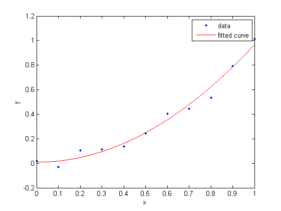
In Matlab, you can fit noisy data using the curve fitting toolbox. Example:

xdata = (0:0.1:1)';               % column vector!
noise = 0.1*randn(size(xdata));
ydata = xdata.^2 + noise;
f = fittype('a*x.^2 + b'); 
fit1 = fit(xdata, ydata, f, 'StartPoint', [1,1])
plot(fit1, xdata, ydata)

Side note: plot() is not our usual plot function, but a method of the cfit-object fit1.

Our fit uses the data to determine the coefficients $a,b$ of the underlying model $f(x) = a x^2 + b$ . We can read out the uncertainty of the coefficients (the "confidence interval" of the coefficients) into a matrix. Each column(!) of the matrix corresponds to one coefficient, with the coefficients alphabetically ordered.

names = coeffnames(fit1)   % check the coefficient order!
ci = confint(fit1, 0.68);  % 1 sigma interval
a_ci = ci(:,1)
b_ci = ci(:,2)

By default, Matlab uses $2 \sigma$ (0.95) confidence intervals. As a physicist, make sure to specify $1 \sigma$ (0.68) intervals.

Confidence and Prediction Bands

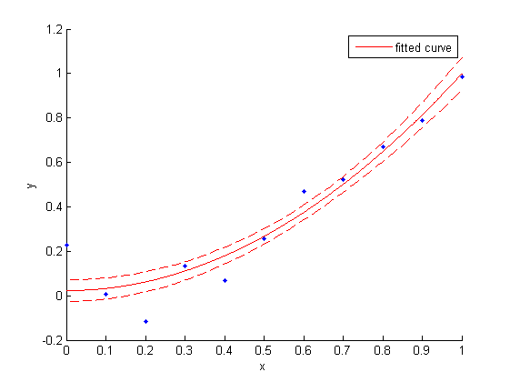
The confidence intervals of the coefficients do not tell the whole story - especially when the coefficients are correlated! A good visualisation of this case is to plot confidence bands or prediction bands around our data.

Prediction band: If I take a new measurement value, where would I expect it to lie? In Matlab terms, this is called the "observation band".
Confidence band: Where do I expect the true value to lie? In Matlab terms, this is called the "functional band".

As with the coefficient's confidence intervals, Matlab uses $2 \sigma$ bands by default, and you should switch it to $1 \sigma$ intervals. By its nature, the prediction band is bigger, because it comprises the uncertainty of the model (the confidence band!) and the scatter of the measurement.

There is a another destinction to make, one that I don't fully understand. Both Matlab and Wikipedia make that distinction.

Pointwise: How big is the prediction/confidence band for a single measurement/true value? In virtually all cases I can think of, this is what you would want to ask as a physicist.
Simultaneous: How big do you have to make the prediction/confidence band if you want a set of all new measurements/all prediction points to lie within the band with a given confidence?

In my personal opinion, the "simultaneous band" is not a band! For a measurement with $n$ points, it should be $n$ individual error bars!

The prediction/confidence distinction and the pointwise/simultaneous distinction give you a total of four options for "the" band around the plot. Matlab makes the $2 \sigma$ pointwise prediction band easily accessible, but what I am usually interested in is the $1\sigma$ pointwise confidence band. It is a bit more cumbersome to plot, because you have to specify dummy data over which to evaluate the prediction band:

x_dummy = linspace(min(xdata), max(xdata), 100);
figure(1); clf(1);
hold all
plot(xdata,ydata,'.')
plot(fit1)    % by default, evaluates the fit over the currnet XLim
% use "functional" (confidence!) band; use "simultaneous"=off
conf1 = predint(fit1,x_dummy,0.68,'functional','off');
plot(x_dummy, conf1, 'r--')
hold off

Note that the confidence band at $x=0$ equals the confidence interval of the fit-coefficient $b$ !

Extrapolation

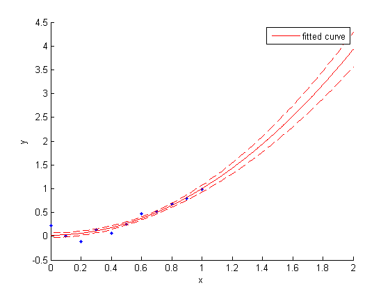
If you want to extrapolate to x-values that are not covered by the range of your data, you can evaluate the fit and the prediction/confidence band for a bigger range:

x_range = [0, 2];
x_dummy = linspace(x_range(1), x_range(2), 100);
figure(1); clf(1);
hold all
plot(xdata,ydata,'.')
xlim(x_range)
plot(fit1)
conf1 = predint(fit1,x_dummy,0.68,'functional','off');
plot(x_dummy, conf1, 'r--')
hold off