notes

previous 2 of 12 Next

dat.gui Minimal Example

Posted on 11 Jun 2016

dat.gui is a small js library to create a widget in the upper right corner of the screen, with which variables can be changed (see examples).

I love how simple this widget is: You specify the variables you want to influence, and based on the each variable type, dat.gui will automatically add the appropriate UI element:

string –> edit field
function –> checkbox
number –> slider (use optional arguments to restrict range)

This is a minimal HTML example on how to use it in a small app with only one variable (see result here):

<!DOCTYPE html>
<html lang="en">
  <head>
    <meta charset=utf-8 />
    <style type="text/css">
      /* style goes here */
    </style>
    <title>dat.gui Test</title>
  </head>
  <body>
    <h1>dat.gui Test</h1>
    <script type="text/javascript" src="dat.gui.min.js"></script>
    <script type="text/javascript">
var MainView = function() {
  this.message = 'hello there';
  this.appContainer = document.createElement('div');
  this.appContainer.innerHTML = this.message;
  document.body.appendChild(this.appContainer);
};

var mainView = new MainView();
var gui = new dat.GUI();
gui.add(mainView, 'message').onFinishChange(function (newText) {
  mainView.appContainer.innerHTML = newText;
});
    </script>
  </body>
</html>

Some small comments, since I have not used JavaScript in ages:

The "main GUI" is defined as a MainView object, which is created with var mainView = new MainView();

The constructor MainView() has lots of internals defined with via the this keyword. This makes these properties accessible to the public, so that dat.gui can see them. It also ensures that they can be changed by other callbacks, etc. It's always a bit confusing what this actually refers to, but since we only create one of these objects, we are pretty much fine either way.

The scripts are placed at the bottom of the body tag (old school) to ensure that document.body exists. Some people view this as bad style, since then the JS is loaded last, but in this case that's OK, since nothing else is deferring loading of the app.

The gui.add(...) defines the meat of the GUI widget. This line includes a callback for what to do when the user entered a new value. Having to define the callbacks like this makes the definition of the widget less clear than often shown in examples. In the online examples, they cheat by shoving the callbacks into the MainView() object (see example here and inspect the source). This is shown in the modified example below. It does make the definition of the GUI look prettier, but I don't like it, because:

The type of callback seems to be limited to onChange, as opposed to something like "onFinishedChange". Typically, I don't want that.
It uses more lines of code.
message is a pseudo-object that also exists as argument of the creator. That's pretty advanced stuff, where scope and this becomes confusing. No thank you - I'd rather stick to the simpler code that is easier to reason about.

In any case, here is the code of the modified example (see result here, should look identical to first example):

<!DOCTYPE html>
<html lang="en">
  <head>
    <meta charset=utf-8 />
    <style type="text/css">
      /* style goes here */
    </style>
    <title>dat.gui Test</title>
  </head>
  <body>
    <h1>dat.gui Test running</h1>
    <script type="text/javascript" src="dat.gui.min.js"></script>
    <script type="text/javascript">
var MainView = function(message) {
  // __defineGetter__ and __defineSetter__ makes JavaScript believe that
  // we've defined a variable 'this.message'. This way, whenever we
  // change the message variable, we can call some more functions.
  this.__defineGetter__('message', function() {
    return message
  });
  this.__defineSetter__('message', function(m) {
    message = m;
    this.changeMessage(m)
  });
  
  this.appContainer = document.createElement('div');
  this.appContainer.innerHTML = message;
  document.body.appendChild(this.appContainer);
  
  this.changeMessage = function(m) {
    this.appContainer.innerHTML = m;
  };
};

var mainView = new MainView('hello again');
var gui = new dat.GUI();
gui.add(mainView, 'message');
    </script>
  </body>
</html>

I came across the dat.gui library while looking at the awesome experiment Texter.

Default Matlab Plot Colors

Posted on 13 Jan 2016

I try to be consistent in my thesis and use the same colors everywhere. Since version 2014b, Matlab has a nice color palette. The RGB values and hex-values for the colors can be output using:

colors = get(0, 'defaultAxesColorOrder');
rgbs = round(256*colors);
hexes = num2str(rgbs, '%02X')

This returns the following values (nicefied into a table by hand):

    R     G     B      hex       name
   ========================================
 114   190    0072BE     blue
  83    25    DA5319     red/orange
 178    32    EEB220     yellow
  47   142    7E2F8E     purple
 173    48    77AD30     green
 191   239    4DBFEF     light blue
  20    47    A3142F     dark red

Since color names are highly debatable, here are the colors, shown from left to right in the default Matlab color order:

If these don't work out, I find that paletton often helps me in finding nice, harmonizing colors.

For quick calculations in Mathematica

Posted on 27 Nov 2015

Some constants that I use almost every time:

V = Quantity[1, "Volts"];
mm = Quantity[1, "Millimeters"];
e = Quantity[1, "ElementaryCharge"];
amu = Quantity[1, "AtomicMassUnit"];
T = Quantity[1, "Teslas"];
Hz = Quantity[1, "Hertz"];

Transforming both sides of an equation in Mathematica

Posted on 12 Aug 2015

Today I tried to manually solve some equations when I realized I had made an error somewhere. So I turned to Mathematica to find the error. I wanted to multiply both sides of my equation by some factors, and to add or subtract some constants from both sides. Bascially, I wanted to do "equivalent transforms" ("Äquivalenzumformung" in German) with Mathematica.

Unfortunately, when doing operations on an equation in Mathematica, the operation does not "thread through" to the left hand side and the right hand side. So I defined these simple functions (careful, no error handling, no cases, no nothing)

eAdd[eq_, const_] := (eq[[1]] + const == eq[[2]] + const) ;
eSub[eq_, const_] := (eq[[1]] - const == eq[[2]] - const) ;
eMul[eq_, const_] := (eq[[1]] * const == eq[[2]] * const);
eDiv[eq_, const_] := (eq[[1]] / const == eq[[2]] / const);
ePow[eq_, const_ ] := (eq[[1]]^const == eq[[2]] const);

The first argument is assumed to be an equation (this is crucial, but not actually checked), the second argument the paramter that should be added/subtracted/divided... Now I can do simple equation transforms:

eq = (5 == 10 - a x);
eq = eAdd[eq, a x];
eq = eSub[eq, 5];
eq = eDiv[eq, a] 
(*-> x == 5/a *)

Again, there is no error checking, and no warning for edge-cases (for instance, a=0 is not checked). It's no replacement to Solve[eq, x].

Another function that came in handy a few times: Expanding a fraction with some factor:

fracExpandWith[fraction_, factor_] := 
 Simplify[Numerator[fraction]*factor]/
  Simplify[Denominator[fraction]*factor]

This is helpful to massage fractions which Mathematica has trouble simplifying:

fracExpandWith[(1/x^2 + 5) / (a + 5/x), x^2]
(*-> (1 + 5 x^2)/(x (5 + a x)) *)

Of course, this function also lacks all safety and sanity checks. Wouldn't be fun, otherwise.

Floating Number Woes

Posted on 22 Jun 2015

The following snippet evaluates to 0 in Mathematica:

fp = 1/2 (fc + Sqrt[fc^2 - 2*fz^2]);
fm = 1/2*(fc - Sqrt[fc^2 - 2*fz^2]);
fp^2 + fm^2 + fz^2 - fc^2 // Simplify

But when you run

fc = 30000000.;
fz = 4000000.;

and evaluate the first bit of code again - the result will be non-zero (on my machine: 0.125).

It took me embarrassingly long to figure out that this was a floating point problem. I have computed this sort of code for the last 5 years, and somehow I must have gotten lucky, because I always computet the last line slightly different:

Sqrt[fp^2 + fm^2 + fz^2] - fc

The way that floating point numbers are stored makes the second version much, much more benign - but for me, such floating points woes are not intuitive yet.

I am somewhat sad that it's 2015 and these problems still sneak up on us. Mathematica should have warned be about this. We've had "modern" interval arithmetic since the 1960s - machines have the power to warn when they might be outputting garbage! (Edit: See bottom of page for why and when Mathematica warns me)

Indeed, you can easily use Intervals in Mathematica (and in Matlab, it's a popular package) to show that the result "0.125" is such garbage:

In Mathematica, you can define arbitrary intervals using the Interval function. When this function is given a single argument, it gives you the smallest Interval that can be represented with standard machine precision. Therefore, define

fc = Interval[30000000.];
fz = Interval[4000000.];

and rerun the first snippet - the result is Interval[{-1.75, 1.875}]. This interval is bigger than the actual error, but this is a deliberate trade-off to guarantee that the true result is within the interval, without having to use brutally complicated math for the proof. You can get a smaller interval by using arbitrary precision numbers, for instance with 200 digits:

fc = Interval[30000000.`200];
fz = Interval[4000000.`200];

Oh well, now I know to be more careful. And instead of complaining I should probably start setting a good example by using Interval arithmetic from the start. It's actually quite simple!

Edit: I just learned why Mathematica did not warn about the garbage that it returned. When using machine-precision numbers (ordinary floating numbers like 1.2), then it does not do any fancy interval arithmetic or precision control with them. This makes the calculations reasonably fast. When using arbitrary precision numbers (like 1.2`20), then Mathematica does reason about the precision and warns about garbage. Normal machine precision is a precision of about 16 decimal digits. When specifying all numbers as 4000000`16, and so on, then Mathematica warns me. This is a speed/convenience trade-off - still, I wish Mathematica was smart enough to see that my calculation costs no time whatsoever and simply rerun it with arbitrary precision numbers to give me a warning...

Bottom line: Instead of using Interval, one can also use arbitrary precision numbers and trust that (hopefully) Mathematica gives more sensible output.

Cleaning stainless steel parts for UHV

Posted on 08 Apr 2015

This is a summary of this document, which is in German. It deals mostly with cleaning 1.4301 stainless steel. I added some bits from personal experience.

You need to know the pumping speed $S$ of your pump. Typical value is $80\,\text{l/s}$ for a small, 2500€ turbo pump. Knowing the pumping speed and the inlet pressure $p$ , you can calculate the pump throughput $Q = S p$ .

In typical UHV applications, the pumps must deal with the leak flow rate $Q_\text{leak}$ .The actual vacuum in far ends of the system then depends on the conductivities $L$ of the pipes. Conductivities are 1/(Resistance) and have the same unit as the pumping speed. Important distinction: Throughput depends on pressure difference: $Q = L \Delta p$

The leak rate $Q_\text{leak}$ can be caused by

mechanical leak: Typical value is $10^{-6}\,\text{mbar}\,\text{l}/\text{s}$ for a hair placed on the O ring of a KF flange. The leak rate can easily be 5 orders of magnitude larger, and you still won't here a hissing sound. You can find $10^{-4}\,\text{mbar}\,\text{l}/\text{s})$ leaks using snoop leak checking fluid. Smaller leaks need a helium leak checker to find. Typically, you can avoid or close leaks.
permeation of gas (helium) through bulk material: Stainless steel parts thicker than a few mm won't have this problem. O rings show leak rates of $10^{-5}\,\text{mbar}\,\text{l}/\text{s})$ when you spray them with helium for more than 20 seconds or so.
diffusion of gases trapped in bulk material to the outside: Hydrogen atoms leak towards the vacuum with typically a few $10^{-12}\,\text{mbar}\,\text{l}/(\text{s}\,\text{cm}^2)$ . Note that I used the area normalized leak rate $q = Q/A$ here. This can be reduced by baking the parts in vacuum.
desorption of material trapped/smudged on the surface. Usual suspects are water, carbohydrates, and heavy metals. A cleaned and baked stainless steel part still outgases water with $10^{-10}\,\text{mbar}\,\text{l}/(\text{s}\,\text{cm}^2)$ , although the exact value depends a lot on the cleaning method.

You are also worried about particles trapped on the surface, from lints of cleaning wipes, dust particles, particles in cleaning water, glove abrasions, ... These particles can be a source of outgasing, they can disturb semi-conductor manufacturing processes, and (relevant for physicists) trap surfaces charges that disturb beam-optics of low energy (<100eV) beams. I am going to neglect particles here: If you want to get serious about them, you need a clean room. Other than that, lint free wipes and deionized (purified) water help a lot.

Countermeasures: Better than cleaning is to avoid contamination. Use only tools, holders, and machining oils that are free of heavy metals when manufacturing the parts. Use deionized (purified) water only. Cleaning helps to combat desorption of surface material and removes particles. Baking helps with surface desorption as well, and with diffusion of gases trapped in the bulk metal.

Coarse cleaning: Pressure washer, wire brush, turning in a lathe, milling until the surface looks nice. Wipe everything down with lint-free wipes.

Fine cleaning: Always clean in ultrasonic bath as the last step. Before that, you can do:

Electro polishing: Using a bath with the right electrolyte and a suitable electrode structure smooths the surface (larger field gradient near edges). Creates a thin chrome-oxide layer that acts as a diffusion barrier for hydrogen. Not too effective in removing hydrocarbons.
Mechanical polishing: Smooths the surface and takes off hydrocarbons with it. Only drawback: Does not create a barrier agains hydrogen diffusion from the bulk.
Bead blasting removes the top surface layer and any hydrocarbons with it. But surface will be rougher compared to electropolishing or mechanical polishing, so expect more outgassing of water. Creates dust particles that are tricky to remove.

After everything is mounted, bake out. Higher is better, 300°C is a bit impractical, but works rather quickly (only a few hours needed).

So much for the suggested procedure. Here is what we do:

Workshop does no polishing of the parts, but machines the surfaces carefully in the last go of the lathe/milling machine. Degreases them using several rounds of ultrasonic bathing and drying in an oven.
We get the parts, and if they are small enough, ultrasound them in a bath of isopropanole, water, and acetone (in no specified order). If they are big, we just wipe them down with isopropanole, then acetone.
We use nitrile gloves to handle the parts and aluminum foil to put them down or to wrap them.
We mount the parts. For technical reasons, we don't go above 120°C when baking. Often we bake at only 50°C for two weeks.

Using a small 80l/s pump on a 1.5m long, stainless steel beamtube with 2cm diameter, and two 8cm diamater, 30cm long chamber on each end, we easily reach $10^{-10}\,\text{mbar}$ and below. Caveat: We measure near the pump - so on the far end of the tube, vacuum is worse. Once we dip the far end into liquid helium, our vacuum is too good to measure. We don't see any ion loss with Carbon4+ or Oxygen5+ ions, and can store single ions over weeks.

Triggering Devices with an Arduino

Posted on 08 Apr 2015

Oscilloscopes, function generators, etc., usually come with a TTL-compatible trigger input. Most of the time, this input takes 5V signals, sometimes 3.3V signals. Typically, the input impedance is not specified. My Agilent arbitrary waveform generator uses 10kOhm input impedance.

TTL-compatible means that the inputs have a high impedance and that, by design, a single microcontroller output should be able to drive several inputs simultaneously (fan out).

How does a typical microcontroller perform as a trigger generator? I am using an Arduino Uno, which can drive 40mA per pin, with a slightly modifight blink example:

void setup() {
  pinMode(12, OUTPUT);
}

void loop() {
  digitalWrite(12, HIGH);   // Pin 13 has internal LED -> Use Pin 12
  delay(1);                 // 2x 1 ms -> 500Hz
  digitalWrite(12, LOW);    
  delay(1);
}

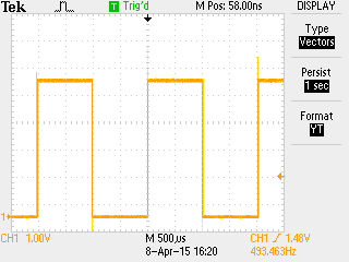
I used clips and 1.5m of 50Ohm BNC cable to connect this to my oscilloscope (which has standard high-impedance inputs). For my measurements I did not connect this signal anywhere else: There was no trigger input listening. But routing this signal further to the TRIG-IN of a function generator did not change its properties too much - most of it was additional ringing caused by the extra cable. The following description applies to both cases.

The rising edge of my ~500Hz signal looks surprisingly clean, considering that the 50Ohm cable is not matched to the output and input impedances of the signal. The slew-rate is between 0.5V/ns and 1.0V/ns, the rise-time 10ns. You see some slight ringing of the cable in the first 100ns.

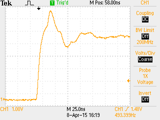
I did not try to measure the exact frequency. My scope gave me a value of 490Hz-495Hz, which I attribute to measurement error of the scope itself.

Looking at the edge of the next period, 2ms later, reveals a surprising amount of jitter. My el-cheapo oscilloscope does not have jitter-analysis software, but my impression was that most jitter is within ±150ns, with occasional spikes up to ±10µs, sometimes even more.

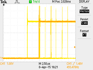
After 10 periods, the jitter got worse by a factor 2 or so.

Overall, using Arduino as a trigger generator seems to work for experiments where several 10µs jitter is OK. In my case, up to 1ms is acceptable, so I went with it.

For demanding applications, it's better to use a proper trigger generator that is designed to drive 50Ohm loads, so that the trigger inputs can be terminated properly. This reduces reflections (ringing). (If you use a 50Ohm driver, you should terminate the signal, otherwise you get twice the voltage!).

In practice, trigger inputs are rarely driven by 50Ohm or terminated properly, because the effects of reflections are very repeatable, which means that they don't matter a lot for the timing.

Cavalier Projection in Matlab and Illustrator

Posted on 28 Mar 2015

When doing quick sketches on paper, I usually use a perspective that I recently learned is called a "cavalier perspective", out of the family of oblique projections.

Unfortunately, Matlab does not support such a perspective natively. But someone on the file exchange wrote a function that enables it. I found it works reasonably nicely with the new graphics system (hg2) of Matlab 2014b.

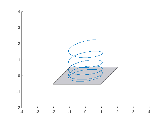
I used a projection angle of 45° for my pictures and a scale factor of 0.50. (30° and 0.5 also works nicely). I exported the graphs to Illustrator for further editing.

In Illustrator, I needed to fake this perspective for a few other elements (arrow-heads and such). In order to be able to do that, I had to jump through some hoops of the UI:

Long-click the scale-tool in the left toolbar, then click on the on the fly-out arrow to make another small toolbar appear. Double-click the scale tool and scale the vertical to 35.2%. Then double-click the shear-tool (mistranslated in the German version as "Verbiegen-Werkzeug") and shear by 45° on a horizontal axis. (Rant: I hate that Adobe still has not discovered the right-click. Seriously. Who long-clicks anything with a mouse? I only found out about this months after I started using Illustrator.)

There are many other oblique projections. I liked this pdf that gives a nice overview. It appears that the naming conventions are subtly different in German and English.

previous 2 of 12 Next